This project focuses on creating a Recurrent Neural Network (RNN) to predict the upcoming faults in a wind turbine based on past failures and general data.
NOTE: the project work stream might be extrapolated, by applying minor modifications and/or fine-tuning procedures, to any new dataset (not limited to wind applications) containing failure information and reach applicable conclusions to real world.
The project is split in the following two parts, covering part 2 in this publication.
Part 1 is focused on next sections:
- INTRODUCTION
- DATA ACQUISITION
- CODE OVERVIEW
- RECURRENT NEURAL NETWORK CREATION
Part 2 is focused on next sections:
- SEQUENCE PREDICTION USING AUTOENCODER
- RNN MULTILABEL
- APPLICATION NETWORK CUSTOMIZATION
As reference, the code is entirely developed in Python using Keras/Tensorflow frameworks and is accessible from below link.
SEQUENCE PREDICTION USING AUTOENCODER
Previous chapter implemented a RNN single-label neural network to predict the next immediate upcoming failure in a wind turbine. However, that approach, in spite of being correct, does not provide a real added value when implemented in a real wind turbine application because failures are asynchronously triggered. Therefore, several failures might be triggered at the same exact timing or with very small delays. Given the project objective is to improve wind turbine cost of quality, predicting the failure to be triggered in the next time instance is not helpful since some reaction time to apply a mitigation action is expected.
In light of the above reasoning, the target should be to provide an overview of the upcoming failures, not just the next immediate failure. To implement that approach, current chapter focuses on creating an autoencoder neural network to predict an upcoming failures sequence. Autoencoder neural network is a sophisticated multi-input neural network with both encoder and decoder data, described as follows.
- Encoder data: it corresponds to the input defined in Chapter 3, which had past IDs data applied through an embedding layer and 5 features input data to capture one hot wind speed, one hot wind turbine power and standardized elapsed time among failures. Then, both data are concatenated prior to be applied to the encoder GRU RNN layer with ReLU as activation function. The output sequence of the encoder layer is disregarded, and instead the output states are stored to be used as input in the decoder layer.
- Decoder data: it is artificially created in the data generator by assigning to zero a tensor of the same shape as target tensor. Then, it is applied to the decoder GRU RNN layer with ReLU as activation function and setting the units internal states according to the stored encoder layer output states.
Decoder output is then applied to a TimeDistributed-Dense layer with 33 neurons corresponding to the number of different failures and softmax as activation function due to the single-label approach for each predicted value in the output sequence. Note a single output Dense layer as in Chapter 3 is no longer valid for autoencoder applications, because it requires the additional TimeDistributed layer to apply the output Dense layer in each timestep of the output sequence. As an example, next picture depicts an autoencoder network diagram with 100-position embedding layer for the past IDs data and using encoder and decoder GRU layers of 128 neurons.

Autoencoder input and target data are yielded through a generator in the form of [input data, past IDs data, input decoder], target data also implemented in the function generator from utils.py by selecting autoencoder input to True.
Optimal tuning defined for the RNN single-label network, depicted below as reference, is used in the autoencoder simulation. Note training, validation and testing splits and loss function weighting approach also keep the same.

A simulation for an output sequence with length of 3 positions is performed, depicting the dynamic loss function during training next. Both training and validation losses follow the same trend validating the proper model fitting with no overfitting.

Next table depicts the metrics results per output sequence position and also the global performance. The prediction for position 1 reaches a very similar performance as the RNN single-label network, but the predictions for position 2 and 3 shows a clear decreasing trend. That behavior is expected because first prediction is based on solid and robust past data, but further predictions are partly based on previous predictions, which leads to a cumulative carryover error.

To demonstrate how the performance degrades in deeper positions of the output sequence caused by the internal carryover error, the test confusion matrix and classification report with the total and class accuracy, precision and F1 score calculations is shown below for the first and third position in the output sequence. It is observed below how the first position in the output sequence reaches a metrics similar to the previous case of RNN single-label, but the third position leads to significantly worse metric results.
POSITION 1 OUTPUT SEQUENCE PREDICTION


POSITION 3 OUTPUT SEQUENCE PREDICTION


As summary, current chapter details an autoencoder neural network implementation to predict an output sequence given a certain input sequence. Each prediction in the output sequence is generated by assessing the immediate past data, considering when needed the previous predicted data. Therefore, this kind of architecture implies a cumulative carryover error for wrong predictions, jeopardizing the accuracy for the following predictions. Note that error is a mandatory cost in some applications as NLP, in which a word needs to be predicted based on the previous words, but other implementations might be assessed if a chronological order is not a real added value for the application under analysis.
RNN MULTILABEL
Previous chapter implemented an autoencoder neural network to predict the upcoming failure sequence in a wind turbine. However, predicting a temporal output sequence implies an intrinsic cumulative carryover error caused to make further predictions based on the already predicted data. That cumulative carryover error cost is mandatory for some application as NLP, but that is in fact an unnecessary cost for a wind turbine application. The project objective is to have additional information about the upcoming errors to provide room to anticipate and improve cost of quality, but it does not require to know the exact failure sequence order. The simple fact to know that a certain failure will be triggered in a future time instance allows enough information to apply mitigation actions to reduce failure effect, independently if there was a different previous failure message.
In light of the above reasoning, the current chapter focuses on a RNN multilabel neural network instead of the previous autoencoder output sequence. Therefore, the target data is neither a single upcoming failure represented as 1D one hot vector as in RNN single label nor an output failure sequence represented as a number of 1D one hot vectors equal to the output sequence length as in RNN autoencoder, but it is basically a list of upcoming failures without any chronological order represented as 1D multi one hot vector. It enables the wind turbine technician to know if the failure will be triggered in the short future to take the corresponding mitigation actions.
The RNN multilabel diagram is exactly the same as the RNN single-label diagram because the main changes are internally in the target generation, as explained in the above paragraph, and in the output Dense layer using sigmoid as activation function. Unlike softmax activation function, sigmoid generates a 0-1 probability for each Dense output neuron, and so it might have so many positive output classes as neurons in the output Dense layer. Next picture depicts a RNN multilabel diagram as reference.

Optimal tuning defined in RNN single-label network, depicted below as reference, is used in the RNN multilabel network simulation. Note training, validation and testing splits and loss function weighting approach also keep the same.

A simulation enabling the three upcoming failures in each sample is performed, depicting the metrics and dynamic loss function results and the test classification report below.

Both training and validation losses follow the same trend validating the proper model fitting with no overfitting.

Test classification report shows a macro average F1 score close to 0.59, but with a macro average TPR 0.51 and macro average precision 0.75. As reference, in the RNN single-label simulation F1 was similar, but both TPR and precision were also around 0.6. The main reason about this deviation in TPR and precision performance is caused due to the intrinsic design for a RNN multilabel network. A RNN single-label network will always output a single positive class due to softmax activation function, even the probabilistic evidence is very limited. However, a RNN multilabel network can output no positive class if the probabilistic evidence of each sigmoid activation function is not higher than the significance threshold (by default, it is defined to 0.5). Therefore, the RNN multilabel network only predicts positive classes with high probabilistic evidence, which implies to make less positive class predictions but with more robust likelihood to be properly predicted. It reflects in terms of metrics as an increase for the false negatives cases and a reduction for the false positives cases, leading to higher precision and lower TPR, as the RNN multilabel results depicts.
As summary, current chapter details a RNN multilabel neural network implementation to predict a list of upcoming failures without any chronological order. Each failure is independently predicted with a specific Dense neuron with sigmoid activation function. Positive classes are predicted when the neuron probability is higher than the significance threshold. Therefore, this architecture implies an intrinsic conservatism to only make positive predictions under significant probabilistic evidence, which improves precision but impacts negatively into TPR. The default significance threshold is defined to 0.5, but it might be customized depending on the false positive and false negative consequences in the application under analysis.
APPLICATION NETWORK CUSTOMIZATION
Previous chapter implemented a RNN multilabel neural network to predict upcoming failures without chronological order in a wind turbine. However, it was observed that performance is very dependent on the significance threshold to predict positive classes. Therefore, best solution is purely dependent on the false positive and false negative consequences in the application under analysis.
In light of the above reasoning, the current chapter focuses on customizing the significance threshold of the RNN multilabel neural network to optimize final application benefits. In the wind turbine application for the project, the consequences of a false positive and false negative prediction are as follows:
- False positive: it will trigger wrong mitigation actions, having a clear negative impact. For example, it might lead to prematurely replace components with the corresponding extra cost or modify turbine operating conditions affecting power production capability to mitigate a non-existing concern or risk.
- False negative: it implies not to have knowledge about the upcoming failures, which has no effect compared to the baseline scenario of not having implemented the neural network model developed in the project.
Therefore, wind turbine application prioritizes having less predictions but with higher precision in the predictions. To implement that strategy, the concept of strong prediction is defined as follows.
- A strong prediction corresponds to the class per each sample with the highest probabilistic evidence if the probability exceeds the significance threshold.
- In case no probability class exceeds the significance threshold, there is no strong prediction for that sample.
- A strong prediction is TRUE if the strong predicted class is among the positive targets of that sample.
- A strong prediction is FALSE if the strong predicted class is not among the positive targets of that sample.
Based on the strong prediction concept, the next in-house metrics are created in the custom_metrics.py file for multilabel applications.
- Multilabel Total Accuracy: accuracy calculated as the total true strong predictions vs the total samples. It reflects the number of samples that the model has properly predicted one of the upcoming failures.
- Multilabel Total Precision/ Relative precision: precision calculated as the total true strong predictions vs total strong predictions. It reflects the number of correct predictions among all predictions made.
- Prediction Ratio: it calculates the percentage of samples with a strong prediction. It reflects the number of samples with a strong prediction, independently on the prediction outcome.
Again, optimal tuning defined in RNN single-label network, depicted below as reference, is used in the RNN multilabel network simulation. Note training, validation and testing splits and loss function weighting approach also keep the same.

Three simulations enabling the three upcoming failures in each sample are performed using different significance threshold in each run. The three significance thresholds are 0.5, 0.7 and 0.85. As reference, next picture depicts the metrics and dynamic loss function results for each simulation. In all cases, both training and validation losses follow the same trend validating the proper model fitting with no overfitting.
SIGNIFICANCE THRESHOLD = 0.5


SIGNIFICANCE THRESHOLD = 0.7


SIGNIFICANCE THRESHOLD = 0.85
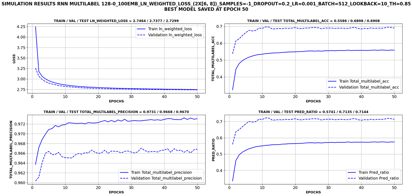


Next table summarizes the results for three different significance thresholds (0.5, 0.7 and 0.85).

The results show a very high values for both macro average precision and relative accuracy in all cases, meaning the model only makes strong predictions under high certainty degree and probabilistic evidence. The higher the significance threshold is, the higher the prediction precision, but at the same time the lower the prediction ratio and total accuracy. Therefore, there is a trade-off between prediction certainty degree and number of predictions made. The optimal trade-off is based on the application under analysis. Thus, if the cost of a false positive is very high, it would be beneficial to increase significance threshold, making less predictions but with higher certainty degree. Instead, if the cost of a false positive is tolerable, lower significance threshold would be recommended to make more predictions with slightly lower certainty degree.
Based on the above described trade-off, the significance threshold must be defined according to a false positive prediction downsides. For a wind turbine application, a false positive has a clear negative impact, and instead, a false negative has null impact. Therefore, the conservative recommendation would be to implement the model with a significance threshold = 0.85, which would predict around 71.5% of the samples with a prediction accuracy of 96.7%. Thus, the false positive consequences are minimized since model will only make predictions under very robust certainty degree. For the remaining 28.5% of the samples, the neural network will not reach enough certainty degree to make a solid prediction and it will not provide information about the upcoming failures, which does not cause any downside since it matches with the baseline scenario of not implementing the developed neural network model.
As summary, current chapter details a RNN multilabel neural network customization to the application under analysis. It has been demonstrated that there is no generic best model or strategies and considering final application is crucial to reach an optimal model maximizing potential benefits.
NEXT STEPS
Future work not captured in these publications for this project might include the following work streams:
- Failure clustering: original dataset had +600 different failures, some of them with only a few occurrences. As the purpose is not really to identify the failure, but it is to define a mitigation action to avoid turbine downtime, failures might grouped depending on the mitigation action to implement when triggered. Different failures will lead to the same mitigation action and splitting them only creates complexity and potential inaccuracy in the neural network.
- Failure mitigation capability assessment: not all failures might be mitigated, even knowing the failure will be triggered in a future time instance. The project pursued a generic approach to reach a better macro average performance, but a failure weight distribution based on mitigation capability might lead to better real field application benefits (in spite of potential worse macro average metrics results).
- Extra input data features: project focuses on main data as power, wind speed or elapsed time, but a wind turbine has thousands of operating signals, which some of them might has a significant correlation to trigger certain failure. Therefore, adding new features might boost model learning power.
I appreciate your attention and I hope you find this work interesting.
Luis Caballero
